Once per window · Flush
Write to the full state
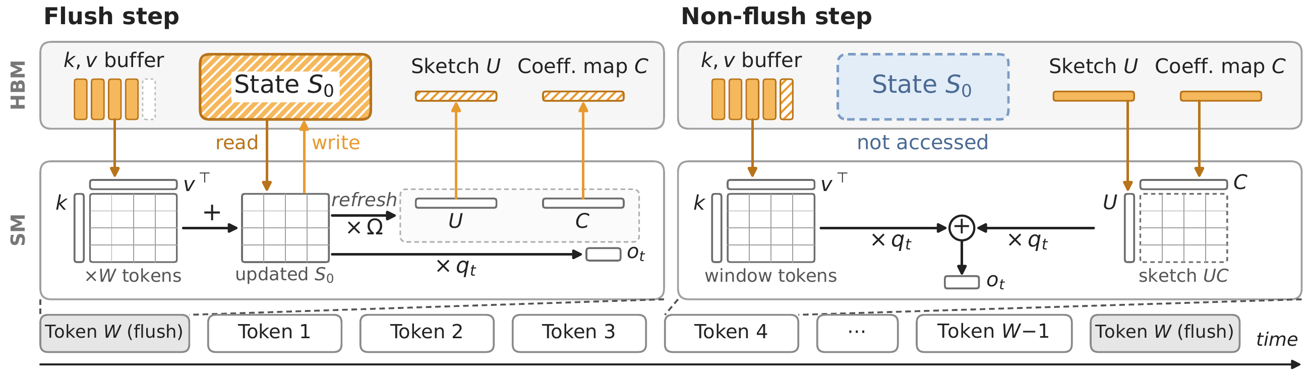
Apply buffered updates to the uncompressed state, then refresh a compact sketch. The state is never replaced with its approximation.
Avoid propagating state-compression errors.*
Write to the Full State,
Read from a Compact Sketch
1Seoul National University2UC Berkeley3KAIST
Co-corresponding authors



SketchSSM decode throughput
faster than the standard baseline
faster than ReplaySSM
| Method | Accuracy (%) | Throughput (tokens/s) | Decode speedup | |||||
|---|---|---|---|---|---|---|---|---|
| IFEval | MATH-500 | HumanEval | MBPP | Average | vs Standard | vs ReplaySSM | ||
| Standard | 86.1 ± 1.3 | 67.7 ± 1.7 | 81.4 ± 2.5 | 71.1 ± 1.9 | 76.6 ± 0.9 | 3,383 | 1.00× | -- |
| ReplaySSM | 85.8 ± 1.3 | 66.4 ± 1.7 | 81.9 ± 2.4 | 70.8 ± 1.9 | 76.2 ± 0.9 | 4,669 | 1.38× | 1.00× |
| SketchSSM | 85.4 ± 1.3 | 67.5 ± 1.7 | 80.9 ± 2.6 | 70.9 ± 1.9 | 76.2 ± 1.0 | 7,634 | 2.26× | 1.64× |
Accuracy is reported as mean ± standard error over problems. Speedups and throughput are from the demo.
01 / The idea
A recurrent state carries information into every future step. Compressing that state can carry approximation errors forward, too. SketchSSM preserves full-state updates and approximates only the readout to avoid propagating state-compression errors into subsequent decoding steps.*
Each update inherits the previous state's error. Compressing the updated state adds a new error term.
Full stateSt = MtSt−1 + Bt
Compressed stateS̃t = Q(MtS̃t−1 + Bt)
Error propagationEt = MtEt−1 + εt
Et = S̃t − St. Mt is the state transition, Bt the new update, Q state compression, and εt the new compression error. This comparison holds the input sequence and update terms fixed to isolate direct state-compression error.
State-write access: Already amortized across multiple decoding steps by ReplaySSM, making full-state updates affordable while avoiding state-compression error propagation.
State-read access: Reduced by reading from a compact sketch refreshed alongside each full-state update.
Once per window · Flush
Apply buffered updates to the uncompressed state, then refresh a compact sketch. The state is never replaced with its approximation.
Avoid propagating state-compression errors.*
Between flushes · Non-flush
Combine sketch vectors with query-dependent coefficients to approximate the state readout. Recent buffered updates contribute separately to the output.
No full-state access between flush steps.
* Readout approximation errors can still propagate through output vectors and affect subsequent full-state updates. Here, avoiding error propagation refers specifically to preventing the accumulation of errors from information discarded by state compression during ring-buffered state updates.
02 / How to Make a Sketch
Within each window, the full state stays fixed, but the effective query changes at every decoding step. Computing each query's output directly therefore requires rereading the same full state.
Our idea is to approximate these changing queries with a small, fixed query basis. A single full-state read at the flush step precomputes the outputs for all basis vectors, forming a compact sketch. Subsequent queries combine these precomputed outputs instead of rereading the full state.
U = [u₁, u₂, u₃] = S0⊤Ω
To choose a basis that preserves the output, we minimize output reconstruction error—equivalently, state-weighted query approximation error.
H = S0S0⊤; S0 is the full state at the window boundary, and q̃t is the effective query incorporating within-window transitions.
Offline · Fixed
Use the average state geometry E0 = 𝔼𝒟[S0S0⊤]. Uncentered PCA of zt = E01/2q̃t gives PG, the top G eigenvectors of 𝔼𝒟[ztzt⊤]. Calibrate once per state head; keep the basis fixed during inference.
Per window · Flush
Refresh U and the state-dependent map C with each full-state update. Sketch construction is fused into the update kernel. Here, † denotes the pseudoinverse; the implementation uses an efficient approximation of C.
Per step · Non-flush
Choose query-dependent coefficients that minimize ∥S0⊤q̃t − Uc∥22, then combine the sketch vectors. Read only the compact sketch and map; the buffered contribution to the output remains exact.
03 / Accuracy
At mean sketch rank Ḡ = 8, SketchSSM preserves average accuracy across four benchmarks for all four models spanning Mamba-2, Gated DeltaNet, and KDA, while reducing state-access traffic by 9.4–10.7× relative to Standard.
Follow the green curves. Moving right means less state traffic; staying high means better accuracy. Pruning and quantization lose accuracy at smaller traffic reductions because errors introduced by state compression propagate across decoding steps.
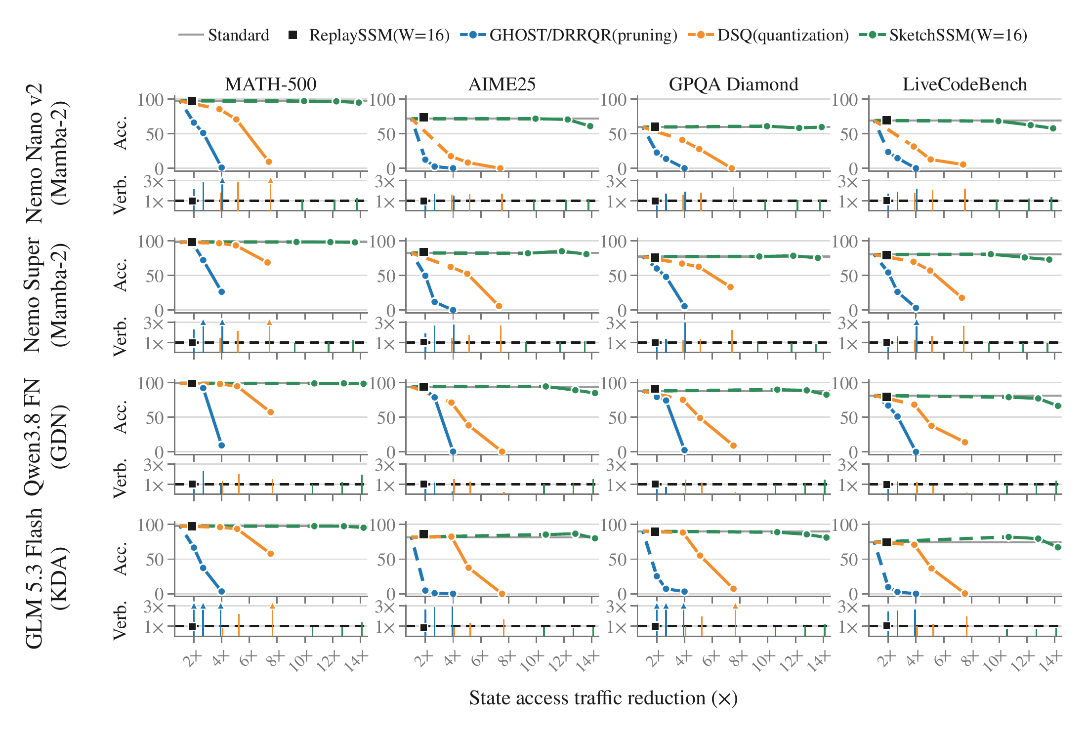
Sketch rank controls the accuracy–traffic trade-off. Larger traffic reductions can decrease accuracy.
04 / Linear-attention kernel speedup
Most steps read only the sketch, not the full state, to reduce memory traffic.
At a flush step, SketchSSM refreshes the sketch by fusing the sketch construction computation into the existing state update kernel.
Nemotron 3 Super
Qwen3.8 Flash-Next
GLM 5.3 Flash
Whole-window kernel speedups over Standard · Mean sketch rank Ḡ = 8 · 1× NVIDIA B300 · W = 16 · Batch 512
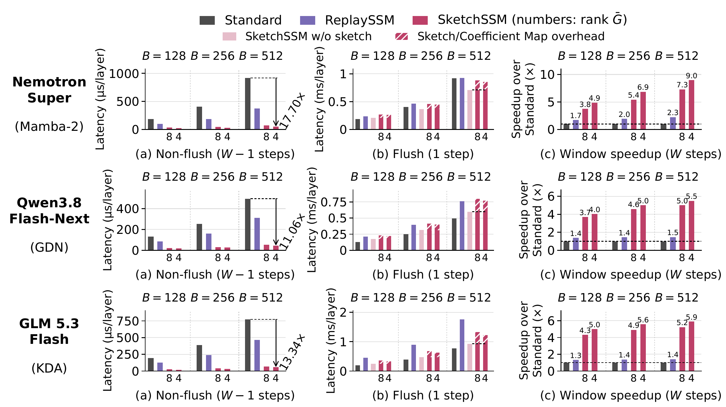
In the paper’s end-to-end evaluation at mean sketch rank Ḡ = 8, these kernel improvements translate to 2.77× higher decode throughput at 2K context and 2.33× at 8K on Nemotron 3 Super with one NVIDIA B300, compared with Standard at each method’s maximum batch size.
Try SketchSSM
vLLM integration, CUDA kernels, evaluation scripts, and ready-to-use calibration files.
 Get started on GitHub
 git clone https://github.com/SNU-ARC/SketchSSM.git
cd SketchSSM/vllm
VLLM_USE_PRECOMPILED=1 python -m pip install -e .
python -m pip install sketchssm # CUDA kernels; without it vLLM uses its Triton kernels Calibrated query bases are available.
 Stay tuned for more models. You can also create your own offline calibration for your model using the SketchSSM code repository.
@misc{kwon2026sketchssmwritestateread,
  title={SketchSSM: Write to the Full State, Read from a Compact Sketch},
  author={Omin Kwon and JoongWon Shin and Minseo Kim and Kurt Keutzer and Sehoon Kim and Jae W. Lee},
  year={2026},
  eprint={2609.33051},
  archivePrefix={arXiv},
  primaryClass={cs.LG},
  url={https://arxiv.org/abs/2609.33051}
}